Note
Go to the end to download the full example code.
Plot Intracranial Electrodes
This notebook demonstrates calculating anatomical information about intracranial electrodes and plotting on the Freesurfer average brain.
# Author: Gavin Mischler
#
# License: MIT

import numpy as np
import matplotlib.pyplot as plt

import naplib as nl
from naplib.localization import Brain
from naplib.visualization import plot_brain_elecs, plot_brain_overlay
Load freesurfer fsaverage data if we don't have it
import os
import mne
os.makedirs('./fsaverage', exist_ok=True)
mne.datasets.fetch_fsaverage('./fsaverage/')
Attempting to create new mne-python configuration file:
/home/docs/.mne/mne-python.json
Could not read the /home/docs/.mne/mne-python.json json file during the writing. Assuming it is empty. Got: Expecting value: line 1 column 1 (char 0)
179 files missing from root.txt in /home/docs/checkouts/readthedocs.org/user_builds/naplib-python/checkouts/latest/examples/brain_plotting/fsaverage
Downloading missing files remotely
Downloading data from 'https://osf.io/download/3bxqt?version=2' to file '/tmp/tmp9xet74j2/temp.zip'.

  0%|                                               | 0.00/196M [00:00<?, ?B/s]
  0%|                                       | 179k/196M [00:00<01:52, 1.74MB/s]
  1%|▍                                     | 2.08M/196M [00:00<00:16, 11.8MB/s]
  5%|█▉                                    | 10.1M/196M [00:00<00:04, 43.0MB/s]
 10%|███▋                                  | 19.0M/196M [00:00<00:02, 60.8MB/s]
 14%|█████▏                                | 26.8M/196M [00:00<00:02, 67.0MB/s]
 18%|██████▊                               | 35.3M/196M [00:00<00:02, 73.2MB/s]
 22%|████████▎                             | 42.7M/196M [00:00<00:02, 73.2MB/s]
 26%|█████████▋                            | 50.0M/196M [00:00<00:01, 73.1MB/s]
 30%|███████████▍                          | 58.8M/196M [00:00<00:01, 77.9MB/s]
 34%|████████████▉                         | 66.9M/196M [00:01<00:01, 78.7MB/s]
 39%|██████████████▋                       | 75.6M/196M [00:01<00:01, 80.9MB/s]
 43%|████████████████▎                     | 83.7M/196M [00:01<00:01, 81.0MB/s]
 47%|█████████████████▉                    | 92.5M/196M [00:01<00:01, 83.1MB/s]
 52%|████████████████████                   | 101M/196M [00:01<00:01, 82.3MB/s]
 56%|█████████████████████▋                 | 109M/196M [00:01<00:01, 80.3MB/s]
 60%|███████████████████████▎               | 117M/196M [00:01<00:00, 80.6MB/s]
 64%|████████████████████████▉              | 125M/196M [00:01<00:00, 76.2MB/s]
 68%|██████████████████████████▍            | 133M/196M [00:01<00:00, 76.0MB/s]
 72%|████████████████████████████           | 141M/196M [00:01<00:00, 77.7MB/s]
 76%|█████████████████████████████▋         | 149M/196M [00:02<00:00, 77.2MB/s]
 80%|███████████████████████████████▍       | 157M/196M [00:02<00:00, 79.6MB/s]
 85%|█████████████████████████████████      | 166M/196M [00:02<00:00, 81.6MB/s]
 89%|██████████████████████████████████▊    | 175M/196M [00:02<00:00, 83.1MB/s]
 94%|████████████████████████████████████▌  | 183M/196M [00:02<00:00, 84.0MB/s]
 98%|██████████████████████████████████████▎| 192M/196M [00:02<00:00, 84.8MB/s]
  0%|                                               | 0.00/196M [00:00<?, ?B/s]
100%|████████████████████████████████████████| 196M/196M [00:00<00:00, 827GB/s]
Extracting missing files
Successfully extracted 179 files
10 files missing from bem.txt in /home/docs/checkouts/readthedocs.org/user_builds/naplib-python/checkouts/latest/examples/brain_plotting/fsaverage/fsaverage
Downloading missing files remotely
Downloading data from 'https://osf.io/download/7ve8g?version=4' to file '/tmp/tmp8f7ktcyo/temp.zip'.

  0%|                                               | 0.00/239M [00:00<?, ?B/s]
  0%|                                       | 170k/239M [00:00<02:20, 1.70MB/s]
  1%|▎                                     | 2.01M/239M [00:00<00:20, 11.5MB/s]
  4%|█▋                                    | 10.5M/239M [00:00<00:05, 45.1MB/s]
  8%|███                                   | 19.4M/239M [00:00<00:03, 62.5MB/s]
 12%|████▌                                 | 28.4M/239M [00:00<00:02, 72.2MB/s]
 16%|█████▉                                | 37.3M/239M [00:00<00:02, 78.1MB/s]
 19%|███████▎                              | 46.3M/239M [00:00<00:02, 82.0MB/s]
 23%|████████▊                             | 55.2M/239M [00:00<00:02, 84.0MB/s]
 27%|██████████▏                           | 64.1M/239M [00:00<00:02, 85.7MB/s]
 31%|███████████▋                          | 73.1M/239M [00:01<00:01, 87.0MB/s]
 34%|█████████████                         | 82.1M/239M [00:01<00:01, 87.8MB/s]
 38%|██████████████▍                       | 91.1M/239M [00:01<00:01, 88.4MB/s]
 42%|████████████████▎                      | 100M/239M [00:01<00:01, 88.8MB/s]
 46%|█████████████████▊                     | 109M/239M [00:01<00:01, 89.1MB/s]
 49%|███████████████████▎                   | 118M/239M [00:01<00:01, 89.2MB/s]
 53%|████████████████████▋                  | 127M/239M [00:01<00:01, 89.4MB/s]
 57%|██████████████████████▏                | 136M/239M [00:01<00:01, 89.5MB/s]
 61%|███████████████████████▋               | 145M/239M [00:01<00:01, 89.3MB/s]
 64%|█████████████████████████              | 154M/239M [00:01<00:00, 89.0MB/s]
 68%|██████████████████████████▌            | 163M/239M [00:02<00:00, 88.9MB/s]
 72%|████████████████████████████           | 172M/239M [00:02<00:00, 88.1MB/s]
 76%|█████████████████████████████▍         | 180M/239M [00:02<00:00, 88.3MB/s]
 79%|██████████████████████████████▉        | 189M/239M [00:02<00:00, 88.5MB/s]
 83%|████████████████████████████████▎      | 198M/239M [00:02<00:00, 86.4MB/s]
 87%|█████████████████████████████████▊     | 207M/239M [00:02<00:00, 87.1MB/s]
 90%|███████████████████████████████████▎   | 216M/239M [00:02<00:00, 87.6MB/s]
 94%|████████████████████████████████████▋  | 225M/239M [00:02<00:00, 83.3MB/s]
 98%|██████████████████████████████████████▏| 234M/239M [00:02<00:00, 85.1MB/s]
  0%|                                               | 0.00/239M [00:00<?, ?B/s]
100%|████████████████████████████████████████| 239M/239M [00:00<00:00, 941GB/s]
Extracting missing files
Successfully extracted 10 files

PosixPath('/home/docs/checkouts/readthedocs.org/user_builds/naplib-python/checkouts/latest/examples/brain_plotting/fsaverage/fsaverage')
Create a brain with the pial surface for computing metrics
brain = Brain('pial', subject_dir='./fsaverage/').split_hg('midpoint').split_stg().simplify_labels()

# Specify the coordinates of 30 electrodes in fsaverage space
coords = np.array([[-47.281147  ,  17.026093  , -21.833099  ],
                   [-48.273964  ,  16.155487  , -20.162935  ],
                   [-51.101261  ,  13.711058  , -16.258459  ],
                   [-55.660889  ,   9.761111  , -12.340655  ],
                   [-58.733326  ,   6.046287  ,  -9.626602  ],
                   [-60.749279  ,   2.233287  ,  -8.044459  ],
                   [-61.26712   ,  -1.939675  ,  -8.582445  ],
                   [-63.686226  , -10.447982  ,  -0.445693  ],
                   [-63.453224  ,  -9.826311  ,   1.095302  ],
                   [-48.792809  ,  15.73144   , -19.34193   ],
                   [-51.336754  ,  13.27527   , -15.57861   ],
                   [-53.301971  ,  11.016301  , -12.48259   ],
                   [-55.044659  ,   9.894337  , -11.228349  ],
                   [-57.597462  ,   6.753941  ,  -8.082416  ],
                   [-60.594891  ,   2.579503  ,  -6.884331  ],
                   [-63.078999  ,  -8.770401  ,  -1.878142  ],
                   [-67.419235  , -26.153931  ,  -1.260003  ],
                   [-60.28742599, -11.71243477,   5.62593937],
                   [-63.12403107, -12.37896156,   4.09772062],
                   [ 64.44213867,  -3.16063929,  -6.95104313],
                   [ 61.58537674, -23.53317833,  -3.20349312],
                   [ 69.31034851, -18.18317795,   1.97798777],
                   [ 69.0439682 , -18.64465904,   1.2625511 ],
                   [ 68.32962799, -20.90372849,  -0.25190961],
                   [ 59.79437256, -23.76178932,  -3.52095652],
                   [-56.57900238,  -9.23060513,  -7.33194447],
                   [-58.861763  , -11.2859602 ,  -6.18047237],
                   [-61.13874054, -11.35863781,  -4.49999475],
                   [-60.82435989,  -8.91696072,  -3.20156574],
                   [-61.00576019,  -7.45676041,  -3.06485367]])

isleft = coords[:,0]<0
Get anatomical labels for each electrode
['mSTG' 'mSTG' 'mSTG' 'mSTG' 'mSTG' 'mSTG' 'mSTG' 'mSTG' 'mSTG' 'mSTG'
 'mSTG' 'mSTG' 'mSTG' 'mSTG' 'mSTG' 'mSTG' 'pSTG' 'mSTG' 'mSTG' 'mSTG'
 'pSTG' 'pSTG' 'pSTG' 'pSTG' 'pSTG' 'mSTG' 'mSTG' 'mSTG' 'mSTG' 'mSTG']
Compute the distance of each electrode from posteromedial HG along the cortical surface
dist_from_HG = brain.distance_from_region(coords, isleft, region='pmHG', metric='surf')
print(dist_from_HG)
[52.67211969 50.86446306 46.6258215  42.63758415 39.27460724 37.07385395
 36.85639736 27.13146072 25.69458138 49.98035531 45.88171027 42.72107443
 41.56546499 37.83171644 35.98377774 28.77996954 32.920761   19.91693572
 22.38750331 36.74425306 41.73006064 30.15477367 30.96079365 33.36495598
 43.59780259 37.00318716 34.83448731 32.22574902 31.71335103 30.79269113]
Smoothly interpolate values over the brain's surface from electrodes
# As an example, we will use the y coordinate of the electrode
values_per_electrode = coords[:,1] - coords[:,1].min()

# Interpolate onto only the temporal lobe, using the 5 nearest neighbor interpolation with
# a maximum distance of 10mm
brain.interpolate_electrodes_onto_brain(coords, values_per_electrode, isleft, roi='temporal', k=5, max_dist=10)

# Plot the overlay for just the left hemisphere
fig, axes = plot_brain_overlay(brain, cmap='Reds', view='lateral', figsize=(12,6), hemi='lh')
plt.show()

Create a brain with the inflated surface for plotting
Plot electrode locations with matplotlib, and color the electrodes by their distance from HG
fig, axes = plot_brain_elecs(brain, coords, isleft, values=dist_from_HG, hemi='lh', view='lateral')
plt.show()

Plot electrodes with an interactive plotly figure, and instead of coloring them by a value, we will color them by a custom color for each electrode. Some common use-cases for this might be to color electrodes based on the identity of the subject they came from when pooling electrodes, or by a categorical variable. In this case, we color them by the anatomical labels they were assigned to (black for posterior STG and red for middle STG)
colors = ['k' if lab == 'pSTG' else 'r' for lab in anatomical_labels]
fig, axes = plot_brain_elecs(brain, coords, isleft, colors=colors, backend='plotly')
fig.write_html("interactive_brain_plot.html") # save as an interactive html plot
fig.show() # show the interactive plot in the notebook
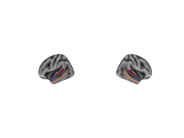
Color certain brain regions by their label
brain.paint_overlay('mSTG', -3)
brain.paint_overlay('pSTG', 3)
brain.paint_overlay('MTG', 1)
fig, axes = plot_brain_overlay(brain, view='lateral')
plt.show()
Plot default Destrieux Atlas region labels overlaid on the brain
brain = Brain('pial', subject_dir='./fsaverage/')

brain.lh.overlay = brain.lh.labels
brain.rh.overlay = brain.rh.labels

fig, axes = plot_brain_overlay(brain, cmap='tab20')
plt.show()

Load and plot Glasser Atlas region labels overlaid on the brain
brain = Brain('pial', atlas='HCPMMP1', subject_dir='./fsaverage/')

brain.lh.overlay = brain.lh.labels
brain.rh.overlay = brain.rh.labels

fig, axes = plot_brain_overlay(brain, cmap='prism')
plt.show()

Total running time of the script: (3 minutes 22.522 seconds)