Banded Ridge: Robustness Check with Null Bands

This example provides a rigorous sanity check for BandedTRF. We insert a "Null Band" (random Gaussian noise) between our meaningful features to ensure the model correctly regularizes irrelevant information.

Robustness Checks included: 1. Stimulus Alignment Visualization. 2. Step-wise Marginal Delta R optimization paths. 3. Order-invariance consistency (Scatter of Order 1 vs Order 2). 4. Kernel weight inspection for noise suppression. 5. Statistical significance via the .summary() method.

import numpy as np
import pandas as pd
import matplotlib.pyplot as plt
from scipy.signal import resample
from scipy.stats import zscore
import naplib as nl
from naplib.encoding import BandedTRF

1. Prepare the Data

Load neural responses to speech and preprocess features. We include speech envelope, peak rate, and a "Null" noise band for validation.

data = nl.io.load_speech_task_data()
n_trials = 3
data = data[:n_trials]

# Standardize neural responses
data['resp'] = nl.preprocessing.normalize(data=data, field='resp')

# Step A: Compute auditory spectrogram and align to modeling rate (100Hz)
spec_fs, feat_fs = 11025, 100
data['spec'] = [nl.features.auditory_spectrogram(trl['sound'], spec_fs) for trl in data]
# Resample spectrogram to match neural response length
data['spec'] = [resample(trial['spec'], trial['resp'].shape[0]) for trial in data]

# Step B: Compute Envelope and Peak Rate (acoustic features)
data['env'] = [zscore(np.sum(trl['spec'], axis=1)) for trl in data]
data['peak_rate'] = [nl.features.peak_rate(trl['spec'], feat_fs, band=[1, 10]) for trl in data]

# Step C: Final alignment and "Null" Noise Injection
# We inject noise to verify that BandedTRF assigns it a high lambda (regularization)
np.random.seed(1)
for i, trial in enumerate(data):
    # Null Band: Gaussian noise scaled to match envelope variance
    noise = np.random.randn(trial['resp'].shape[0])
    data[i]['noise'] = (noise / np.std(noise)) * np.std(data[i]['env'])

WARNING: Resampling audio from 11.025KHz to 16KHz
WARNING: Resampling audio from 11.025KHz to 16KHz
WARNING: Resampling audio from 11.025KHz to 16KHz

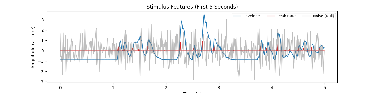
2. Visualize Stimulus Features

Check the temporal alignment of the envelope, peak rate, and injected noise.

fig, ax = plt.subplots(figsize=(12, 3))
t = np.arange(500) / feat_fs
ax.plot(t, data[0]['env'][:500], label='Envelope', color='#1f77b4')
ax.plot(t, data[0]['peak_rate'][:500], label='Peak Rate', color='#d62728')
ax.plot(t, data[0]['noise'][:500], label='Noise (Null)', color='#7f7f7f', alpha=0.5)
ax.set_title('Stimulus Features (First 5 Seconds)')
ax.set_xlabel('Time (s)')
ax.set_ylabel('Amplitude (z-score)')
ax.legend(loc='upper right', fontsize='small', ncol=3)
plt.show()

3. Fit Models with Injected Noise (Order Dependency)

BandedTRF uses a greedy, step-wise approach. We test if the order of feature entry affects the final predictive performance.

tmin, tmax, sfreq = -0.2, 0.5, 100
alphas = np.logspace(-2, 8, 11)

# Fit Model 1: Envelope -> Noise -> Peak Rate
order_1 = ['env', 'noise', 'peak_rate']
model1 = BandedTRF(tmin=tmin, tmax=tmax, sfreq=sfreq, alphas=alphas)
model1.fit(data=data, X=order_1, y='resp')

# Fit Model 2: Peak Rate -> Noise -> Envelope
order_2 = ['peak_rate', 'noise', 'env']
model2 = BandedTRF(tmin=tmin, tmax=tmax, sfreq=sfreq, alphas=alphas)
model2.fit(data=data, X=order_2, y='resp')

Optimizing env:   0%|          | 0/11 [00:00<?, ?it/s]
Optimizing env:  64%|██████▎   | 7/11 [00:00<00:00, 69.84it/s]


Optimizing noise:   0%|          | 0/11 [00:00<?, ?it/s]
Optimizing noise:  18%|█▊        | 2/11 [00:00<00:00, 14.69it/s]
Optimizing noise:  45%|████▌     | 5/11 [00:00<00:00, 15.10it/s]
Optimizing noise:  64%|██████▎   | 7/11 [00:00<00:00, 14.11it/s]
Optimizing noise:  82%|████████▏ | 9/11 [00:00<00:00, 13.62it/s]
Optimizing noise: 100%|██████████| 11/11 [00:00<00:00, 13.34it/s]


Optimizing peak_rate:   0%|          | 0/11 [00:00<?, ?it/s]
Optimizing peak_rate:   9%|▉         | 1/11 [00:00<00:01,  7.66it/s]
Optimizing peak_rate:  18%|█▊        | 2/11 [00:00<00:01,  6.49it/s]
Optimizing peak_rate:  36%|███▋      | 4/11 [00:00<00:00,  7.92it/s]
Optimizing peak_rate:  45%|████▌     | 5/11 [00:00<00:00,  7.55it/s]
Optimizing peak_rate:  55%|█████▍    | 6/11 [00:00<00:00,  6.22it/s]
Optimizing peak_rate:  64%|██████▎   | 7/11 [00:01<00:00,  6.62it/s]
Optimizing peak_rate:  82%|████████▏ | 9/11 [00:01<00:00,  7.98it/s]
Optimizing peak_rate:  91%|█████████ | 10/11 [00:01<00:00,  5.86it/s]
Optimizing peak_rate: 100%|██████████| 11/11 [00:01<00:00,  6.37it/s]


Optimizing peak_rate:   0%|          | 0/11 [00:00<?, ?it/s]
Optimizing peak_rate:  45%|████▌     | 5/11 [00:00<00:00, 45.05it/s]


Optimizing noise:   0%|          | 0/11 [00:00<?, ?it/s]
Optimizing noise:   9%|▉         | 1/11 [00:00<00:01,  8.88it/s]
Optimizing noise:  36%|███▋      | 4/11 [00:00<00:00,  8.72it/s]
Optimizing noise:  45%|████▌     | 5/11 [00:00<00:00,  7.55it/s]
Optimizing noise:  73%|███████▎  | 8/11 [00:00<00:00,  7.98it/s]
Optimizing noise:  82%|████████▏ | 9/11 [00:01<00:00,  7.27it/s]
Optimizing noise: 100%|██████████| 11/11 [00:01<00:00,  6.33it/s]


Optimizing env:   0%|          | 0/11 [00:00<?, ?it/s]
Optimizing env:   9%|▉         | 1/11 [00:00<00:03,  3.22it/s]
Optimizing env:  27%|██▋       | 3/11 [00:00<00:01,  6.73it/s]
Optimizing env:  36%|███▋      | 4/11 [00:00<00:01,  6.74it/s]
Optimizing env:  45%|████▌     | 5/11 [00:00<00:00,  6.93it/s]
Optimizing env:  64%|██████▎   | 7/11 [00:01<00:00,  6.39it/s]
Optimizing env:  82%|████████▏ | 9/11 [00:01<00:00,  7.22it/s]
Optimizing env:  91%|█████████ | 10/11 [00:01<00:00,  6.71it/s]
Optimizing env: 100%|██████████| 11/11 [00:01<00:00,  6.90it/s]

BandedTRF(alphas=array([1.e-02, 1.e-01, 1.e+00, 1.e+01, 1.e+02, 1.e+03, 1.e+04, 1.e+05,
       1.e+06, 1.e+07, 1.e+08]),
          sfreq=100, tmax=0.5, tmin=-0.2)

In a Jupyter environment, please rerun this cell to show the HTML representation or trust the notebook.
On GitHub, the HTML representation is unable to render, please try loading this page with nbviewer.org.

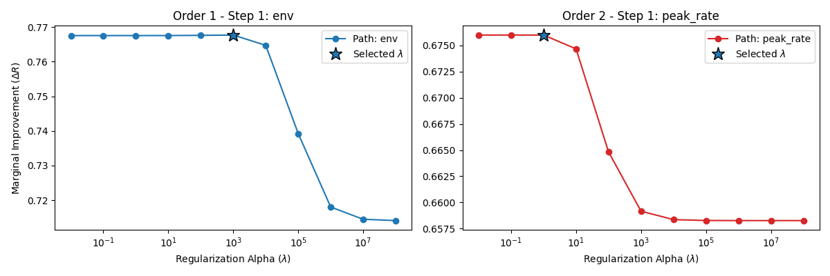
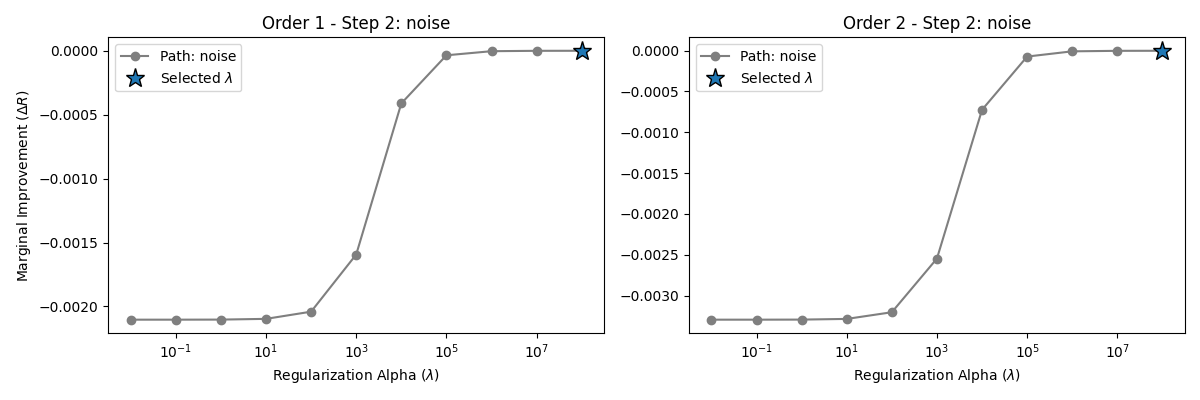
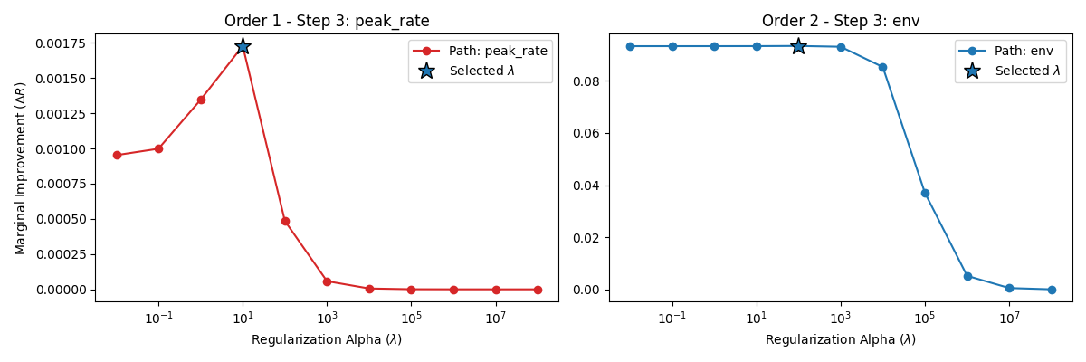
4. Alpha Optimization Paths (Marginal Delta R)

Visualize how much each feature adds to the correlation (r) at each step. For the noise band, we expect a flat or negligible marginal improvement.

colors = {'env': '#1f77b4', 'noise': '#7f7f7f', 'peak_rate': '#d62728'}
n_bands = len(order_1)

for b_idx in range(n_bands):
    fig, axes = plt.subplots(1, 2, figsize=(12, 4), sharey=False)
    for i, (mdl, ord_list) in enumerate(zip([model1, model2], [order_1, order_2])):
        feat = ord_list[b_idx]
        path = mdl.alpha_paths_[b_idx]

        # Calculate Delta R Path relative to the max R of the previous band
        prev_r = 0 if b_idx == 0 else np.max(mdl.alpha_paths_[b_idx-1])
        delta_path = path - prev_r

        best_alpha = mdl.feature_alphas_[b_idx]
        peak_delta = np.max(delta_path)

        axes[i].semilogx(alphas, delta_path, marker='o', color=colors[feat], label=f'Path: {feat}')
        axes[i].plot(best_alpha, peak_delta, '*', markersize=14, markeredgecolor='k', label=r'Selected $\lambda$')
        axes[i].set_title(f'Order {i+1} - Step {b_idx+1}: {feat}')
        axes[i].set_xlabel(r'Regularization Alpha ($\lambda$)')
        axes[i].legend()

    axes[0].set_ylabel(r'Marginal Improvement ($\Delta R$)')
    plt.tight_layout()
    plt.show()

• 
• 
• 

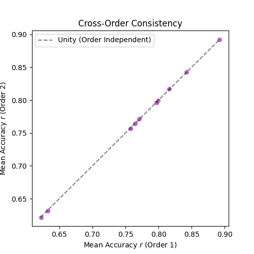
5. Global Consistency: Order 1 vs Order 2

A robust banded model should yield similar final predictive accuracies regardless of the order in which features were added.

r_full_1 = model1.scores_[:,:,-1].mean(axis=0)
r_full_2 = model2.scores_[:,:,-1].mean(axis=0)

fig, ax = plt.subplots(figsize=(5, 5))
ax.scatter(r_full_1, r_full_2, s=50, alpha=0.6, edgecolors='w', color='purple')
# Set limits based on data range
min_r = min(r_full_1.min(), r_full_2.min())
max_r = max(r_full_1.max(), r_full_2.max())
lims = [min_r, max_r]
ax.plot(lims, lims, 'k--', alpha=0.5, label='Unity (Order Independent)')
ax.set_title('Cross-Order Consistency')
ax.set_xlabel('Mean Accuracy $r$ (Order 1)')
ax.set_ylabel('Mean Accuracy $r$ (Order 2)')
ax.legend()
plt.show()

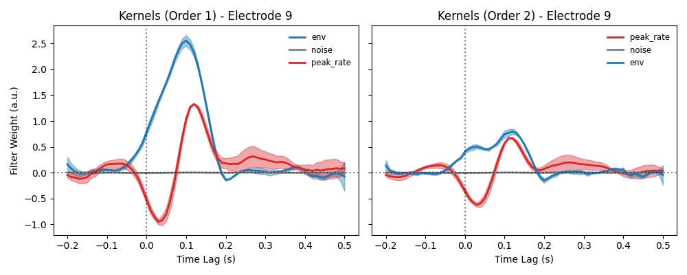
6. Final Model Kernels for the Best Channel

Inspect temporal response functions (TRFs). The 'noise' band TRF should be close to zero, while 'env' and 'peak_rate' should show clear peaks.

best_ch = np.argmax(r_full_1)
fig, axes = plt.subplots(1, 2, figsize=(10, 4), sharey=True)
lags = np.linspace(tmin, tmax, model1._ndelays)

for i, (mdl, ord_list, title) in enumerate(zip([model1, model2],
                                               [order_1, order_2],
                                               ['Kernels (Order 1)', 'Kernels (Order 2)'])):
    for f_idx, feat in enumerate(ord_list):
        # Plot TRF with error shading across trials/CV folds
        nl.visualization.shaded_error_plot(
            lags, mdl.coef_[best_ch, f_idx, :],
            ax=axes[i], color=colors[feat],
            plt_args={'label': feat, 'lw': 2}
        )

    axes[i].axhline(0, color='black', alpha=0.5, linestyle=':')
    axes[i].axvline(0, color='black', alpha=0.5, linestyle=':')
    axes[i].set_title(f"{title} - Electrode {best_ch}")
    axes[i].set_xlabel('Time Lag (s)')
    axes[i].legend(fontsize='small', frameon=False)

axes[0].set_ylabel('Filter Weight (a.u.)')
plt.tight_layout()
plt.show()

# Statistical Significance Summary for the most responsive electrode
print(f"\nFinal Statistics for Model 1 (Order: {order_1}), Electrode {best_ch}:")
model1.summary(best_ch)

print(f"\nFinal Statistics for Model 2 (Order: {order_2}), Electrode {best_ch}:")
model2.summary(best_ch)

Final Statistics for Model 1 (Order: ['env', 'noise', 'peak_rate']), Electrode 9:

BandedTRF Summary | Channel 9
----------------------------------------------------------------------
          Total R Delta R    Alpha     t-value   p-value
Feature
env        0.8902  0.8902 1.00e+03  163.850999  0.000019
noise      0.8902  0.0000 1.00e+08    0.936419  0.223955
peak_rate  0.8923  0.0021 1.00e+01    6.428857  0.011676

Final Statistics for Model 2 (Order: ['peak_rate', 'noise', 'env']), Electrode 9:

BandedTRF Summary | Channel 9
----------------------------------------------------------------------
          Total R Delta R    Alpha     t-value   p-value
Feature
peak_rate  0.7829  0.7829 1.00e+00  119.061810  0.000035
noise      0.7829 -0.0000 1.00e+08   -3.446125  0.962565
env        0.8924  0.1096 1.00e+02   13.875257  0.002577

	Total R	Delta R	Alpha	t-value	p-value
Feature
peak_rate	0.782873	7.828730e-01	1.0	119.061810	0.000035
noise	0.782873	-6.825626e-08	100000000.0	-3.446125	0.962565
env	0.892444	1.095713e-01	100.0	13.875257	0.002577